Backpropagation: Multivariate Chain Rule

Computation graph, chain rule, multivariate chain rule

Introduction

Backpropagation is a core method to perform optimization in Machine Learning. It is commonly used alongside with gradient descent algorithm, which is explained in my previous post.

This is a series of posts on backpropagation. In this post (part 1), we will explore computation graphs, the chain rule, and the multivariate chain rule with visualizations.

1. Backpropagation: Multivariate Chain Rule [Part 1, This post]

2. Backpropagation: Forward and Backward Differentiation [Part 2]

3. Backpropagation: Differentiation Rules [Part 3]

4. Backpropagation: Feed forward network [Part 4]

Some knowledge of derivatives and basic calculus is required to follow these posts.

Derivative and Computation Graph

Let’s take F(x)=x^2 as an example. The function F(x) can be represented with a computation graph:

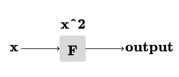
The above computation graph takes x as the input and produces F(x) as the output. In most cases, it is not important what is the content of the node (F) in the computation graph. The nodes are abstractions. A node takes one or more inputs and produces an output.

The derivative of F(x)=x^2 is F’(x)=2x. From the calculus class we know that the definition of the derivative is:

\(F'(x)=\lim_{dx\to0}\frac{F(x+dx)-F(x)}{dx}\)

By rearranging the terms we have:

\(F(x+dx)=F(x)+F'(x) \cdot dx\)

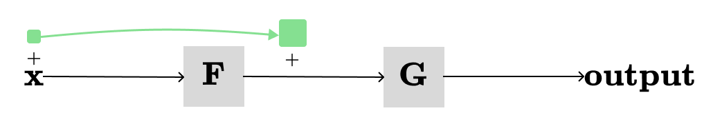
As dx approaches 0, we can use the derivative to closely estimate F(x+dx). One way to visualize our derivative in the same computation graph is:

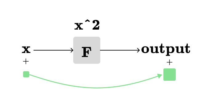
When we add a tiny amount (shown by the smaller green square) to the input x, the output of F(x) is changed by a different amount, represented by the larger green square.

Let’s say the smaller green square above represents dx = 1, then we need two smaller and two larger green squares when dx=2:

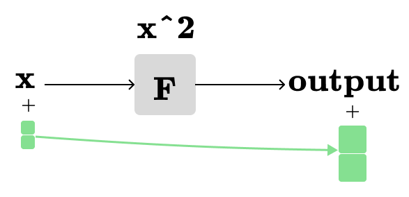
We will need fractional green squares, when dx is less than 1, and so forth. In other words, when we multiply the smaller green square by a scalar, the larger square is also scaled by the same scalar. Additionally, the output rectangle can take on a negative value, indicating subtraction rather than addition. For simplicity, we will use addition in all visualizations, but you should keep in mind that the output rectangle can indeed have a negative value.

Chain Rule

The chain rule is the basis of the backpropagation. In summary, if we have h(x)=f(g(x)) then the chain rule states that:

\(h'(x)=f'(g(x))g'(x)\)

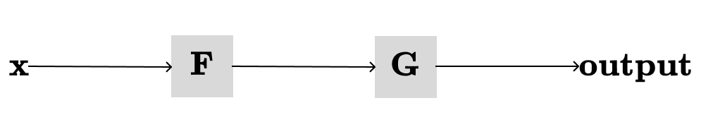
Let’s understand the chain rule with visualizations. Assume we have two functions: F(x)=x^2 and G(x)=3x+5. It is easy to find the derivatives of our functions individually: F’(x)=2x and G’(x)=3. But what is the derivative of their composition G(F(X))?

The composition G(F(X)) can be represented in the computation graph as following:

First let’s visualize the derivative of F with respect to its input x:

The above visualization shows how much the output of F changes (approximately) when a tiny amount (dx=1 in this case) is added to its input x. Let’s do the same for G:

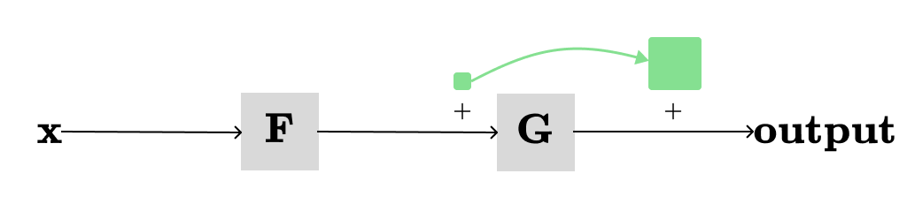
This time, we’re not directly concerned with x, but we’re showing how much the output of G changes when dx=1 is added to its immediate input, which is the output of F.

Next, we want to understand the changes in the overall output when x is changed by dx.

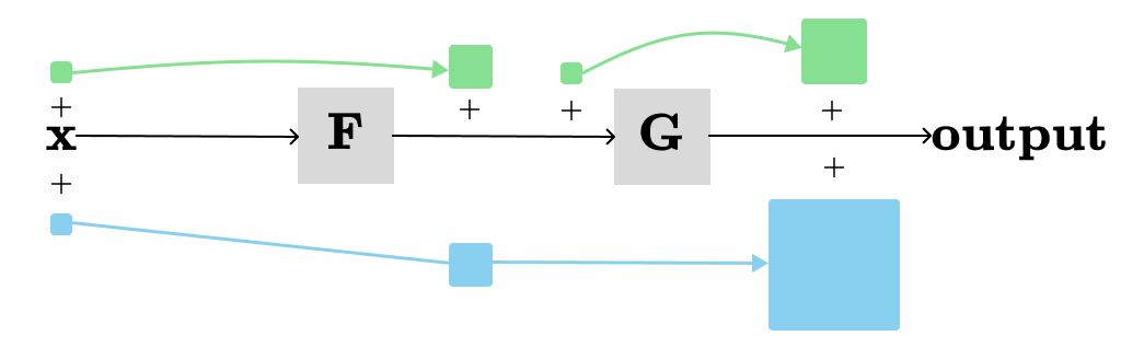
When we adjust x by a small amount, it causes a change in the output of F, which then leads to a change in the output of G (described by the blue path). Note that the larger the change in F's output, the greater the change in G's output. We can observe that the total change in the output resulting from a change in x is simply the product of all local derivatives along the path from x → output. This rule also works when more than two nodes in the path from x → output. Basically, we restated the chain rule.

Multivariate Chain Rule

I find it quite confusing that many tutorials link the chain rule with the backpropagation, instead they should be linking the multivariate chain rule. In this section, we will visualize the multivariate chain rule to gain a better understanding.

First, let’s give a formal definition from the calculus class. Suppose we have some function H(F(x), G(x)), which depends on other functions F and G. Then, the multivariable chain rule allows us to differentiate H with respect to the x:

\(\frac{\mathrm{d}H}{\mathrm{d}x}= \frac{\partial{H}}{\partial{F}}\frac{\mathrm{d}F}{\mathrm{d}x} + \frac{\partial{H}}{\partial{G}}\frac{\mathrm{d}G}{\mathrm{d}x}\)

The function H(F(x), G(x)) together with F(x), G(x) can be represented in the computation graph as following:

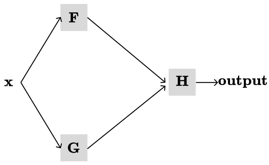
Then, we need to define local derivatives with respect to their immediate input:

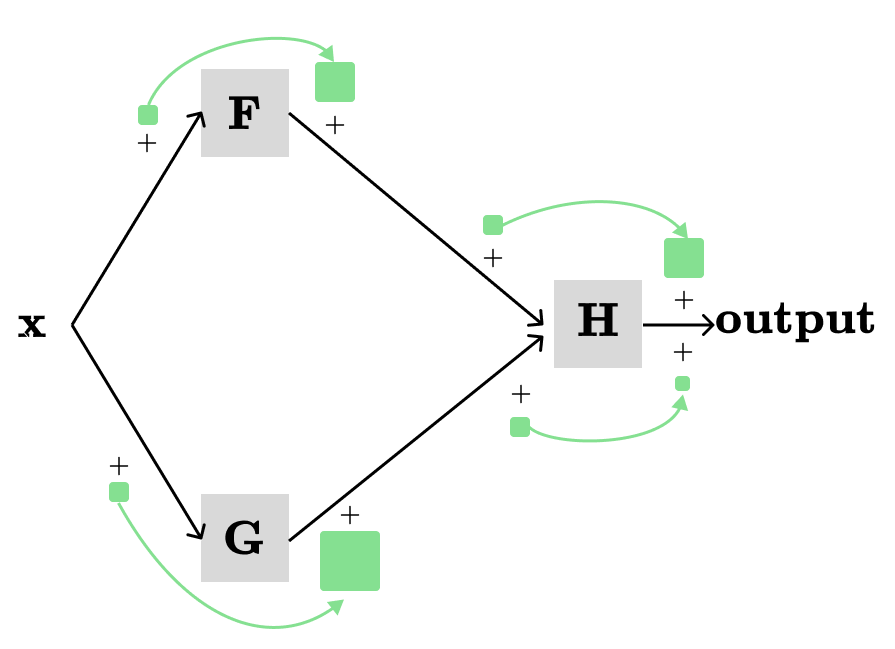
The green squares and arrows show local derivatives of respective functions. Next, we want to show the total contributions to the output from all paths in the graph when we change x a little bit.

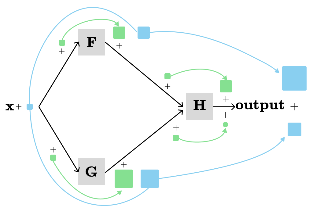
The total contribution is visualized by the blue path. In this example, two different paths contribute to the output, with each path providing the product of all local derivatives along its nodes in the path. Generally, we need to add the products of local derivatives from all the paths from x → output.

The End

This concludes the part 1 of the backpropagation series. Subscribe for the next posts on the backpropagation.