Backpropagation: Differentiation Rules

Derive differentiation rules from scratch with computation graph

Introduction

Backpropagation is a core method to perform optimization in Machine Learning. It is commonly used alongside with gradient descent algorithm, which is explained in my other post.

This is a series of posts on backpropagation. In this post (part 3), we will derive differentiation rules from scratch with computation graph.

The previous posts are prerequisites for this post. Please read them first if you haven't already:

1. Backpropagation: Multivariate Chain Rule [Part 1]

2. Backpropagation: Forward and Backward Propagation [Part 2]

3. Backpropagation: Differentiation Rules [Part 3, This post]

4. Backpropagation: Feed forward network [Part 4]

Some knowledge of derivatives and basic calculus is required to follow these posts.

Differentiation Rules

In the previous posts, we used a computation graph to understand the chain rule and the multivariate chain rule. One nice property of a computation graph is that it enables us to break down a complex function into simpler ones. This breakdown allows us to derive differentiation rules from scratch using a computation graph. Deriving the rules from scratch is fun, and it is also a great way to deepen our understanding of the concepts we've covered so far, such as computation graphs, partial derivatives, and total derivatives.

Constant Rule

Let F(x) = c, where c is a constant that is independent of x, then dF/dx = 0. It is very trivial to proof. We will sometimes use the alternative notation F’(x) for dF/dx.

Let F(x) = c*x, then F’(x)=c, which is derived by:

\(\begin{align} F(x+dx)&= c \cdot (x + dx) \\ &= c \cdot x + c \cdot dx \\ &= F(x) + c \cdot dx \\ &= F(x) + F'(x) \cdot dx \\ \end{align}\)

Let F(x) = x + c, then F’(x)=1, which is derive by:

\(\begin{align} F(x+dx)&= x+dx+c \\ &= F(x) + 1 \cdot dx \\ &= F(x) + F'(x) \cdot dx \\ \end{align}\)

In a general scenario, if F(x) = k*x + c, then it follows that F’(x) = k. It can be proved in a similar way.

Sum Rule

Let H(F(x), G(x))=F(x)+G(x), we want to find dH/dx (or H’(x)):

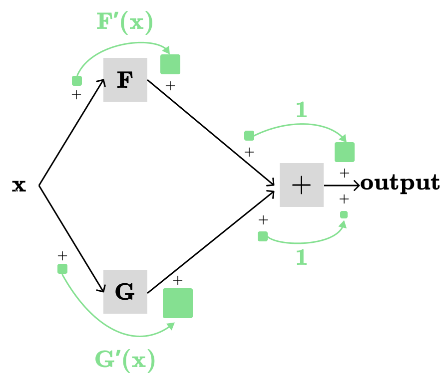
The partial derivatives of the sum, i.e., H(F, G)=F+G, with respect to any of its parameters are always 1, meaning ∂H/∂F and ∂H/∂G are both 1. We already proved this using the rule for F(x)=x+c. Then, the total derivative H’(x) is the sum of products of partial derivatives along the two different paths (see the picture above), which are:

1. x → F → H → output: F’(x) * 1

2. x → G → H → output: G’(x) * 1

which nicely gives us:

\(\begin{align} \frac{\mathrm{d} H(x)}{\mathrm{d} x} &= \frac{\mathrm{d} \left[F(x)+G(x)\right]}{\mathrm{d} x}\\ &= \frac{\mathrm{d} F(x)}{\mathrm{d} x}+\frac{\mathrm{d} G(x)}{\mathrm{d} x}\\ &=F'+G' \end{align}\)

We can combine the constant rule F(x)=c*x with the sum rule to prove linearity:

\(\begin{align} \frac{\mathrm{d} \left[aF(x)+bG(x)\right]}{\mathrm{d} x} &= a\frac{\mathrm{d} F(x)}{\mathrm{d} x}+b\frac{\mathrm{d} G(x)}{\mathrm{d} x}\\ &=aF'+bG' \end{align}\)

As well as the difference rule:

\(\begin{align} \frac{\mathrm{d} \left[F(x)- G(x)\right]}{\mathrm{d}x} &= \frac{\mathrm{d} \left[F(x)+ (-1)\times G(x)\right]}{\mathrm{d} x}\\ &= \frac{\mathrm{d} F(x)}{\mathrm{d} x}+ (-1)\times \frac{\mathrm{d} G(x)}{\mathrm{d} x}\\ &=F'- G' \end{align}\)

Product Rule

Let H(F(x), G(x))=F(x) * G(x), we want to find dH/dx:

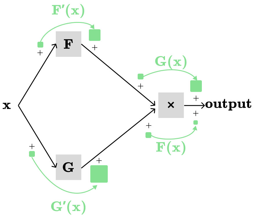
The partial derivatives of H(F(x), G(x))=F(x)*G(x) are:

1. ∂H(x)/∂F(x)=G(x)

2. ∂H(x)/∂G(x)=F(x)

The above partial derivatives are easily derived from F(x)=c*x (see the constant rule section), since we keep the other non-varying parameters constant.

As usual, we have two distinct paths, each contributing to the total derivative:

1. x→F→H→output: F’(x) * G(x)

2. x→G→H→output: G’(x) * F(x)

which gives us the product rule:

\(\begin{align} \frac{\mathrm{d} H(x)}{\mathrm{d} x} &= \frac{\mathrm{d} \left[F(x) \times G(x)\right]}{\mathrm{d} x}\\ &= \frac{\mathrm{d} F(x)}{\mathrm{d} x}G(x) + \frac{\mathrm{d} G(x)}{\mathrm{d} x}F(x)\\ &=F'G+G'F \end{align}\)

Power Rule

Let’s begin with the product rule stated above: H(F(x), G(x)) = F(x) * G(x). This gives us H’(x) = F’(x)G(x) + F(x)G’(x). If we use identity functions for F and G, we get F(x) = x, G(x) = x, and H(x) = x^2. From the product rule F’(x)G(x)+F(x)G’(x), we can derive:

\(H'(x)=F'(x)G(x)+F(x)G'(x)= x'\times x + x \times x' = 2x\)

Amazing, this demonstrates that we can still break down a complex function into simpler ones, even when those simpler functions share the same variable. By extending the product rule to n parameters we can derive the power rule for H(x)=x^n:

\(\begin{align} H'(x)= x' x \dots x + x x' \dots x + \cdots + x x \dots x' = nx^{n-1} \end{align}\)

For the sake of completeness, let’s visualize a more general version of the power rule: H(F(x)) = F(x)^n

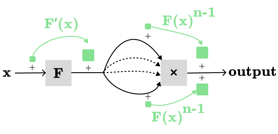
In the computation graph above, we have n different paths, where each path contributing: F’(x)F(x)^(n-1). Hence:

\(\begin{align} \frac{\mathrm{d} H(x)}{\mathrm{d} x} &= \frac{\mathrm{d} [F(x)^n]}{\mathrm{d} x}\\ &=nF(x)^{n-1}\frac{\mathrm{d}F(x)}{\mathrm{d}x}\\ &=nF^{n-1}F' \end{align}\)

Reciprocal Rule

What is the total derivative of G(x)=1/F(x) with respect to the x?

This time we’re going to use the computation graph differently. Let’s introduce another function H(x)=F(x)*G(x). It is easy to see that H(x)=1, since H(x)=F(x)*G(x)=F(x)*(1/F(x))=1. We already know that dH/dx=0 from the constant rule, and we can also express dH/dx as following:

\(\begin{align} \frac{\mathrm{d} H(x)}{\mathrm{d} x} &= \frac{\mathrm{d}F(x)}{dx} \frac{\partial H(x)}{\partial F(x)} + \frac{\mathrm{d}G(x)}{dx} \frac{\partial H(x)}{\partial G(x)} \end{align}\)

The following terms are known to us:

1. dH/dx = 0

2. ∂H/∂F=G(x)=1/F(x) (from F(x)=x*c)

3. ∂H/∂G=F(x) (from F(x)=x*c)

So we have:

\(\begin{align} 0 &= \frac{\mathrm{d}F(x)}{dx} \frac{1}{F(x)} + \frac{\mathrm{d}G(x)}{dx} F(x) \end{align}\)

which gives us:

\(\begin{align} \frac{\mathrm{d}G(x)}{dx} &= -\frac{1}{F(x)^2} \frac{\mathrm{d}F(x)}{dx}\\ &=-\frac{1}{F^2}F' \end{align}\)

Quotient rule

What is the total derivative of H(x)=G(x)/F(x) with respect to the x?

We can compose the quotient rule with the product rule:

\(\begin{align} \frac{\mathrm{d}H}{\mathrm{d}x} &=\frac{\mathrm{d}\left[G(x)\times \frac{1}{F(x)}\right]}{\mathrm{d}x}\\ &=\frac{\mathrm{d}G(x)}{\mathrm{d}x}\frac{1}{F(x)} + G(x)\frac{\mathrm{d}[\frac{1}{ F(x)}]}{\mathrm{d}x}\\ &= \frac{\mathrm{d}G(x)}{\mathrm{d}x}\frac{1}{F(x)} + G(x)\frac{-1}{F(x)^2}\frac{\mathrm{d}F(x)}{\mathrm{d}x}\\ &= \frac{1}{F(x)^2}\left(\frac{\mathrm{d}G(x)}{\mathrm{d}x}F(x) - \frac{\mathrm{d}F(x)}{\mathrm{d}x}G(x) \right) \\ &=\frac{G'F - F'G}{F^2} \end{align} \)

The End

This concludes the part 3 of the backpropagation series. Subscribe for the next posts on the backpropagation.