Backpropagation: Forward and Backward Propagation

Learn about partial and total derivatives, forward and backward propagation

Introduction

Backpropagation is a core method to perform optimization in Machine Learning. It is commonly used alongside with gradient descent algorithm, which is explained in my other post.

This is a series of posts on backpropagation. In this post (part 2), we will explore partial and total derivatives, forward and backward propagation.

1. Backpropagation: Multivariate Chain Rule [Part 1]

2. Backpropagation: Forward and Backward Propagation [Part 2, This post]

3. Backpropagation: Differentiation Rules [Part 3]

4. Backpropagation: Feed Forward Network [Part 4]

Some knowledge of derivatives and basic calculus is required to follow these posts.

Partial and Total Derivatives

In the previous post, we visualized the multivariate chain rule for H(F(x), H(x)) and their derivatives in the same computation graph as following:

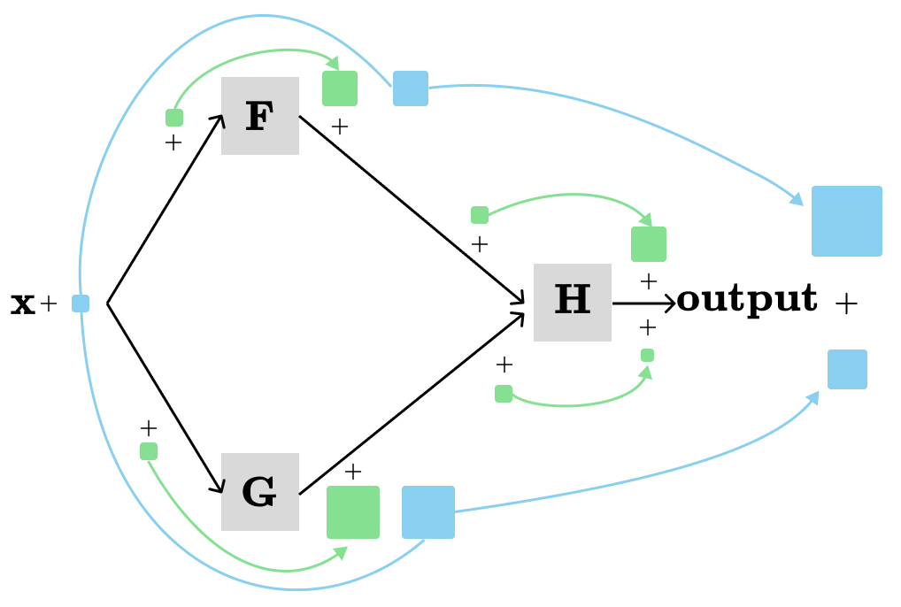
The local derivatives (visualized with green) are called partial derivatives. A partial derivative is only concerned about a single immediate parameter of a single node while the other parameters are held constant. The derivative that describes the total contribution (visualized with blue) is called the total derivative. The total derivative is concerned about all contributions from all different paths in the computation graph.

Let’s revise the formula for the multivariate chain rule:

\(\frac{\mathrm{d}H}{\mathrm{d}x}= \frac{\partial{H}}{\partial{F}}\frac{\mathrm{d}F}{\mathrm{d}x} + \frac{\partial{H}}{\partial{G}}\frac{\mathrm{d}G}{\mathrm{d}x}\)

By examining the formula, you can observe that two distinct notations are used for derivatives: d (total derivative) and ∂ (partial derivative).

It makes sense to use d (total derivative) on the left side because we're interested in the overall effect on H's output when we make a small increase to x, and dH/dx precisely represents that.

What about on the right side? In our simple example, we can interchange d and ∂ without affecting the result. However, d and ∂ will be different in more complex scenarios. For example:

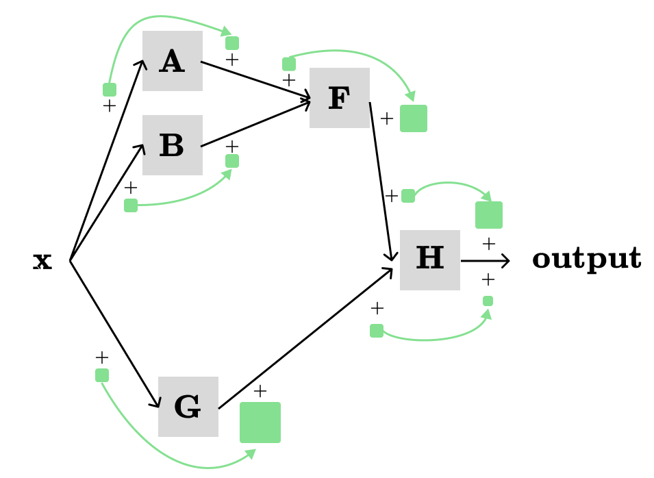
For the computation graph above, the total derivative of H with respect to x (i.e., dH/dx) will be the sum of the products of the partial derivatives along the three different paths:

1. x → A → F → H → output: ∂A/∂x * ∂F/∂A * ∂H/∂F

2. x → B → F → H → output: ∂B/∂x * ∂F/∂B * ∂H/∂F

3. x → G → H → output: ∂G/∂x * ∂H/∂G

By summing the three products we have:

\(\frac{\mathrm{d}H}{\mathrm{d}x}= \frac{\partial{A}}{\partial{x}} \frac{\partial{F}}{\partial{A}} \frac{\partial{H}}{\partial{F}} + \frac{\partial{B}}{\partial{x}} \frac{\partial{F}}{\partial{B}} \frac{\partial{H}}{\partial{F}} + \frac{\partial{G}}{\partial{x}} \frac{\partial{H}}{\partial{G}} \)

The issue with simply summing over the paths is that it can quickly lead to a combinatorial explosion in the number of potential paths.

Luckily, there is a more concise way to express the same thing with less computation. First, we can start by rearranging the terms:

\(\frac{\mathrm{d}H}{\mathrm{d}x}= \frac{\partial{H}}{\partial{F}} \left( \frac{\partial{A}}{\partial{x}} \frac{\partial{F}}{\partial{A}} + \frac{\partial{B}}{\partial{x}} \frac{\partial{F}}{\partial{B}} \right) + \frac{\partial{G}}{\partial{x}} \frac{\partial{H}}{\partial{G}} \)

The term inside the bracket simplifies to dF/dx, so we have:

\(\frac{\mathrm{d}H}{\mathrm{d}x}= \frac{\partial{H}}{\partial{F}}\frac{\mathrm{d}F}{\mathrm{d}x} + \frac{\partial{H}}{\partial{G}}\frac{\mathrm{d}G}{\mathrm{d}x}\)

Note that in this case, we can't substitute dF/dx with ∂F/∂x because they represent different concepts. However, we can interchange dG/dx and ∂G/∂x since they are equivalent.

Additionally, we need to calculate (recursively) dF/dx in the same way as we calculated dH/dx.

Forward Propagation

In the general case, we can ignore most part of the computation graph and only concentrate one a single node (H) and its immediate inputs (F1, F2, …, Fn) at a time:

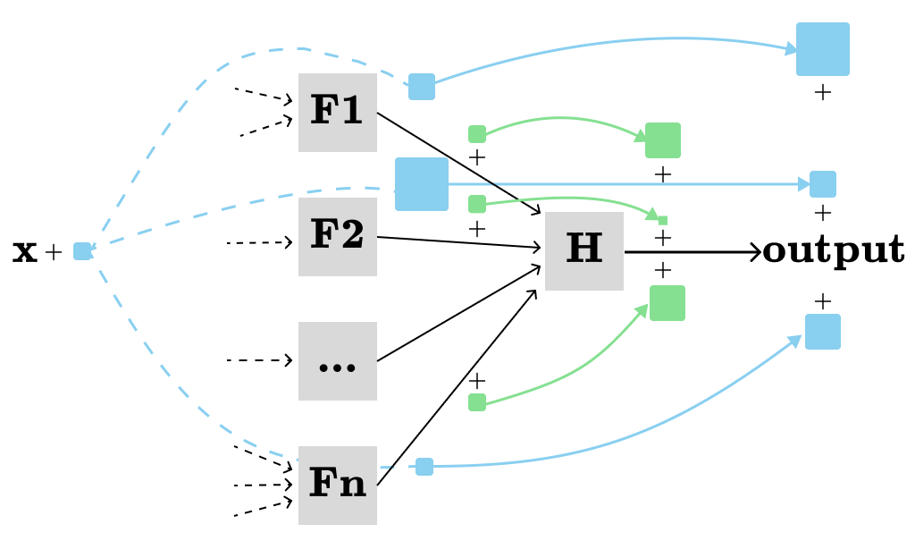
and use the following formula:

\(\frac{\mathrm{d}H}{\mathrm{d}x}= \sum_{i=1}^n \frac{\mathrm{d}F_i}{\mathrm{d}x} \frac{\partial{H}}{\partial{F_i}} \)

Note that we need to compute (recursively) dF[i]/dx in the same way we computed dH/dx.

This formula allows us to efficiently calculate the total derivative of all nodes with respect to a single parameter (x in our case). We can either calculate the total derivatives of nodes by topologically sorting them first or dynamic programing applied on the computation graph. In both cases, we need to ensure that the total derivative of each node with respect to the x (dNode/dx) is computed only once.

The time complexity of the forward propagation is O(V+E), where E is the number of edges and V is the number of nodes in the computation graph. Here, we assume that the time complexity of each individual node (function) is O(1).

Backward Propagation

Forward propagation allows us to efficiently compute the total derivatives of all nodes with respect to a single parameter. However, in machine learning, we usually want to efficiently compute the total derivatives of a single node (the loss output) with respect to all parameters. Backward propagation allows us to achieve this.

Let’s bring back one of our example:

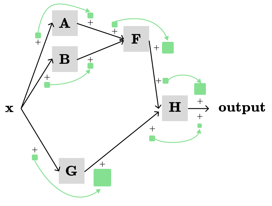
With forward propagation, we were able to efficiently compute the following derivatives:

\(\frac{\mathrm{d}x}{\mathrm{d}x}, \frac{\mathrm{d}A}{\mathrm{d}x}, \frac{\mathrm{d}B}{\mathrm{d}x}, \frac{\mathrm{d}G}{\mathrm{d}x}, \frac{\mathrm{d}F}{\mathrm{d}x}, \frac{\mathrm{d}H}{\mathrm{d}x},\)

With backward propagation, we can instead efficiently compute:

\(\frac{\mathrm{d}H}{\mathrm{d}H}, \frac{\mathrm{d}H}{\mathrm{d}G}, \frac{\mathrm{d}H}{\mathrm{d}F}, \frac{\mathrm{d}H}{\mathrm{d}A}, \frac{\mathrm{d}H}{\mathrm{d}B}, \frac{\mathrm{d}H}{\mathrm{d}x},\)

For example, to compute dH/dx we use the following formula:

\(\frac{\mathrm{d}H}{\mathrm{d}x}= \frac{\partial{A}}{\partial{x}} \frac{\mathrm{d}H}{\mathrm{d}A} + \frac{\partial{B}}{\partial{x}} \frac{\mathrm{d}H}{\mathrm{d}B} + \frac{\partial{G}}{\partial{x}} \frac{\mathrm{d}H}{\mathrm{d}B}\)

Similar to the forward propagation, we can either calculate the total derivatives of nodes by reversed topological order or dynamic programing applied on the computation graph. In both cases, we need to ensure that the total derivative of the output node with respect to the each node (dOutput/dNode) is computed only once.

The time complexity of the backward propagation is O(V+E), where E is the number of edges and V is the number of nodes in the computation graph. Here, we assume that the time complexity of each node (function) is O(1).

The End

This concludes the part 2 of the backpropagation series. Subscribe for the next posts on the backpropagation.