Backpropagation: Feedforward Neural Network

Backpropagation for feedforward neural network from scratch in Python

Introduction

Backpropagation is a core method to perform optimization in Machine Learning. It is commonly used alongside with gradient descent algorithm, which is explained in my other post.

This is a series of posts on backpropagation. In this post (part 4), we will implement backpropagation for feedforward neural network from scratch in Python.

The previous posts are prerequisites for this post. Please read them first if you haven't already:

1. Backpropagation: Multivariate Chain Rule [Part 1]

2. Backpropagation: Forward and Backward Propagation [Part 2]

3. Backpropagation: Differentiation Rules [Part 3]

4. Backpropagation: Feedforward Neural Network [Part 4]

Some knowledge of derivatives and feedforward neural network is required to follow these posts.

Recap

A feedforward neural network is one of the most fundamental neural network architectures, where data flows in a single direction—from the input layer through the hidden layers to the output layer, without looping back.

Since feedforward neural networks are extensively explained in many tutorials and books, I won’t repeat the same information here. If you're not already familiar with this concept, I recommend reviewing it before moving forward with the rest of this post.

The feedforward neural network is usually visualized as following:

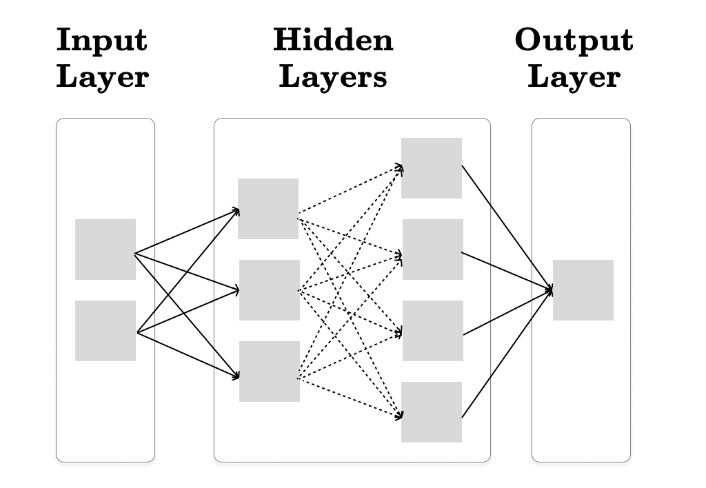
The sample feedforward neural network consists of the following:

• Input Layer: This layer receives two real numbers (x₁, x₂) in our sample neural network. In the general case, it can accept any number of inputs.

• Output Layer: The output layer produces the final output of the model. In this tutorial, we assume that the output is a single real number, which represents the loss of our model. In other words, we want to minimize this value with backpropagation.

• Hidden Layers: These layers consist of one or more similar layers. Each hidden layer applies weighted sum of its inputs followed by a non-linear activation function.

However, I find this visualization confusing because it doesn’t clearly visualize the parameters of our model—the parameters are hidden in the edges of the computation graph. Additionally, the feedforward network could be simplified further by expressing it through basic matrix operations. For these reasons, I prefer the new updated visualization below:

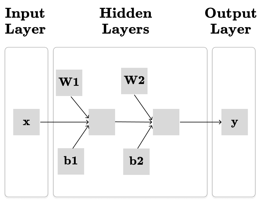
Now, we have:

• x - the input represented with a vector (x ∈ R² in our example)

• y - the output is a single real number (y ∈ R)

• W1, W2 - the weights of the hidden layers are compactly represented by a matrix of size [in_features, out_features], where in_features is the size of the input vector and out_features is the size of the output vector.

• b1, b2 - the bias vectors. A bias is represented with a vector of size out_features.

Each hidden layer in a neural network processes its input using the following logic:

def hidden(input, weight, bias, activation):
    # `input` : a vector of shape (N)
    # `weight` : a 2D matrix of shape (N, M)
    # `bias` : a vector of shape (M)
    # Output : a vector of shape (M)
    # × - matrix multiplication
    return activation(input × weight + bias) 

Using the method described above, we can outline a feedforward neural network in pseudo-code as follows:

def feedforward(x, weight1, bias1, weight2, bias2):
    output = hidden(x, weight1, bias1)
    output = hidden(output, weight2, bias2)
    return output

Note that we use activation functions to introduce non-linearity to the neural network. We will use ReLU in this post. The optimizable parameters of our network are W1, W2, b1 and b2.

Forward Pass

We will develop a feedforward neural network in a modular way, similar to PyTorch’s interface but simplified version of it. The full implementation can be found at https://github.com/maitbayev/mininn and an example jupyter notebook that trains a MNIST model.

First let’s define the Parameter class that holds a numpy array and its gradient:

import numpy as np

class Parameter:
    def __init__(self, value: np.ndarray):
        self.value = value
        self.grad: Optional[np.ndarray] = None

    def accumulate_grad(self, delta: np.ndarray):
        if self.grad is None:
            self.grad = delta
        else:
            self.grad += delta

Then, we define an abstract Module class which roughly represents an abstract Node in our computation graph that we defined in previous posts:

class Module(ABC):
    @abstractmethod
    def forward(self, *inputs: Any, **kwargs: Any) -> Any:
        pass

    @abstractmethod
    def backward(self, *gradients: Any, **kwargs: Any) -> Any:
        pass

    def parameters(self, recurse: bool = True) -> Iterable[Parameter]:
        return iter([])

Let’s also define Sequential module similar to PyTorch’s Sequential class:

class Sequential(Module):
    def __init__(self, modules: list[Module]):
        super().__init__()
        self.modules = modules

    def forward(self, input: np.ndarray) -> np.ndarray:
        output = input
        for module in self.modules:
            output = module(output)
        return output

    def backward(self, gradients: np.ndarray) -> np.ndarray:
        # we will implement later
        ...

    def parameters(self, recurse: bool = True) -> Iterable[Parameter]:
        if recurse:
            for module in self.modules:
                for param in module.parameters():
                    yield param

Please also take a look at the forward pass for ReLU and Linear. I think, they’re self explanatory and straight-forward.

Once setting everything up, we can define our feedforward neural network as follows:

model = mininn.Sequential([
    mininn.Linear(28 * 28, 200),
    mininn.ReLU(),
    mininn.Linear(200, 20),
    ...
])

Backward Pass

During the backward pass, we calculate the total derivative of y with respect to the parameters W1, W2, b1, b2, etc… If you're familiar with matrix calculus, it can be used here. Otherwise, don’t worry! Matrix calculus is not different than regular calculus, it just expresses derivatives more compactly using matrices.

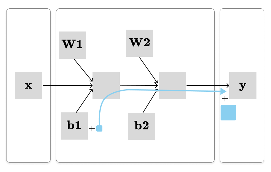
Let’s say we want to calculate the dy / db1, which is visualized above. To achieve this, we calculate the product of partial derivatives along the path from b1 → y. However, it gets quickly confusing if we compute the partial derivatives directly. Because, the partial derivatives of a function f from x ∈ Rⁿ to f(x) ∈ R^m is represented by Jacobian matrix, denoted J_f ∈ R^m×n, where (i,j)^th entry is:

\(J_f[i, j] = \frac{\partial f(x)_i}{\partial x_j}\)

The Jacobian matrix is even more complicated for partial derivatives of W1 and W2, since it will be a tensor of rank 3. We want to avoid this complexity.

We know that the final output is just a single real number (y ∈ R). Therefore, the Jacobian matrix of the total derivative of y with respect to each parameter has the same shape as the parameter itself. Hence, it is far easier to calculate the total derivative of y. We can use an approach called pullback:

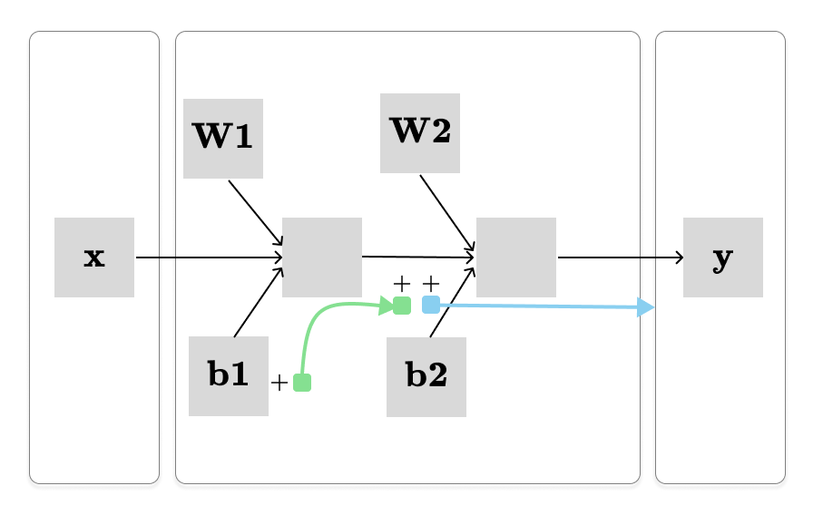
We begin with the total derivative described by the blue path, then pull it back along the green path ( by multiplying by the partial derivative) to obtain the total derivative of y with respect to the b1.

Earlier we defined Module abstract class:

class Module(ABC):
    ...
    
    @abstractmethod
    def backward(self, *gradient: Any) -> Any:
        pass
    
    ...

The backward method receives a gradient parameter that represents the total derivative of y with respect to the module’s output (illustrated by the blue path in the last picture). It should then pullback this gradient backward to compute and return the total derivative of y with respect to the module’s input.

It is more clearer from the Sequential.backward implementation:

class Sequential(Module):
    def backward(self, gradients: np.ndarray) -> np.ndarray:
        output = gradients
        for module in reversed(self.modules):
            output = module.backward(output)
        return output

Take a look at backward implementations of ReLU and Linear as well. They involve a few matrix operations, but nothing especially challenging.

We can see that thinking in computation graphs makes it super easy to build each function on its own and then just plug them together with Sequential.

The End

This concludes the part 4 of the backpropagation series. Subscribe for the next posts.